Introduction
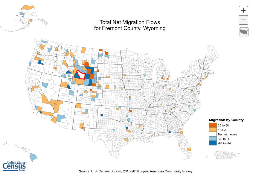
Estimating fine-level migration trends is an important part of allocating resources to ensure long-term projects, such as building infrastructure, are placed optimally to benefit the population that may be growing or shrinking in response to other large scale events. Analyses of local migration trends and impacts are fairly common as the data is fairly easy to attain. A recent study by Badger et al (2021) showed how the local data revealed a trends in migration into politically polarized communities. When it comes to holistic migration data in the U.S. the Census Bureau county to county migration flows represents some of the most fine-grained details that are publicly available. As can be seen from the graphic below this fine level data reveals significant geographically separated patterns, while most migration is obviously from within inner-state counties, on the national level counties can be interconnected without immediately obvious patterns. In this a paper a model is proposed representing national migration impact on county level immigration based on underlying political demographics as a partial explanation for the patterns.
Background Literature
The existing literature for multi-level migration analysis utilizing political characteristics can be largely divided into three broad categories, articles that deal primarily with creating predictions on migration generally, those dealing with the analysis of the effects of migration at various scales, and finally those that identify and isolate political characteristics as a determining factor in migration.
In spatial demography there has long been an interest in predicting migration trends in order to support the appropriate allocation of resources. When it comes to creating models for predicting migration, Tarver (1961) postulated that there were a number of variables that could be taken into account for migration. In his case study of migration in the District of Columbia among individuals he created a model in which “The model posits a disparity in the demographic, economic, and social characteristics among the areas of the country” (Tarver 1961, p. 207) and that areas would evolve those characteristics at different rates. Those characteristics can then be determined to be the driving factor that creates migration disparity and when utilized in a model can be used to create predictions on where migration flow will be directed. Tarver noted that among those three general characteristics there are a potentially exhaustive number of variables that can be utilized which further complicates the model and makes it more difficult to ascertain useful information. In order to fix issues with the multitude of variables, he accounted for “an interaction among the independent variables” (p. 209) within his linear regression model by grouping them into their categories and calculating their effect on each other. Overall Tarver’s model for predicting migration is heavily focused on accounting for a large number of variables and is centered around studying a specific location/time. Drawing from this research it can be concluded that spatially predictive models should strive to reduce or combine similar variables in order to improve their robustness.
More generally there are other models that can be used to describe migration with more aggregate units, such as the gravity model, described as the rule that “any form of spatial interaction (migration, commuting, trade, information exchange, etc.) has the property of flows being positively related to stocks, whichever way measured, and inversely related to distance” (Poot et al 2016, p. 1). One attribute to the gravity model is the idea of distance decay that is not covered in Tarver’s earlier model. When it comes to using the gravity model along with additional characteristic information Poot et al note that “The key constraint to using such additional variables in an augmented gravity model is that in order to derive population projections from the model, forecasts (or assumptions about the future values) of these additional variables will be required” (p.10) Given this constraint the predictive powers of the gravity model are essentially limited to historical data. Using distance as a variable in a multi-level model can be seen as more reliable in this case because the distance projections can be based upon aggregate level predictions which may be easier to generate than for smaller measurement units.
Given the prevalence of migration in demography, it is unsurprising that there is a number of studies of migration captured at various scales and through the multi-level lens as well. McHugh and Grober (1992) capture inter-state migration through time using short interval data (years). Their study notes that “migration researchers have recognized that the magnitude and re-distributive power of migration varies over time.” (p. 429) indicating that variables for migration models can change depending on the environmental conditions. They noted that certain interactions in migration flow could only be fully examined in the context of shorter time frames, such as “During times of economic prosperity migration increased in volume and the system became more integrated in the sense that states exchanged with a wide variety of other states focusing their interactions on one another.” (p. 431) One of the other important observations they made about the level of analysis was that, “California, for example, registered shifts in migration efficiency of 10 percent or more with respect to 32 states, 12 in a positive direction and 19 in a negative direction. California's relative stability in overall migration efficiency (Ej) throughout the 1980s (modest positive) masks major restructuring in the geography of the state's migration connections.” (p. 441) showing that the direction, destination and source are important to maintain during analysis.
Truly delving into the idea of multi-level migration, Dennet and Wilson (2013) explore the relationship between inter-regional and inter-country migration flows throughout Europe. In their article “A new multi-level spatial interaction model is proposed which incorporates data at both country and regional levels in Europe to produce estimates of the inter- regional inter-country flows” (p. 2) Their model thus relies on having access to data for both levels of analysis. One of the observations that they make in their data collection is that “Whilst there are high correlations between these distributions for in-migration, demonstrated across Europe from Census and register data, a ‘capital city effect’ persists where these destinations can attract up to 10% more migrants internationally than internally.” (p. 38) indicating a relationship based upon distance, such as in the gravity model, that can interfere with the characteristics that they are attempting to measure, especially since they are dealing with aggregate rather than individual units. In the culmination of their model they note that “Model (vi) constrains inter-regional estimates to know (but also estimated) inter-country flows allowing us to explore the likely inter-regional international flows within Europe.” (p. 39) indicating that their model is successful in extrapolating characteristics from one level of analysis in order to predict migration flow at another level. Overall this model is very similar to one that could be conducted using county and state level units within the U.S., although it does not include much in the way of other descriptive variables.
Lastly we can look at the literature dealing specifically with narrowing on the political characteristics related to migration, starting with Lam (2002) who points to obvious impact of politics on migration through the “extreme case of refugees leaving a country to escape political persecution.” (p. 489) Lam focuses mainly on how to isolate political factors for migration from other potential factors such as economics, and attempts to determine the value in doing so. She conducts her research on the migration data from Hong Kong and notes that “In our model, the greater the anticipated loss in political freedom and economic stability in the country of origin, the larger the propensity to out-migrate” (p. 492) showing how political events can encourage changes in migration flow. After accounting for the separation of economic and political factors she found that “the incremental effect of having no political confidence on emigration is higher than that of having no economic confidence” (p. 500), emphasizing the importance of incorporating political characteristics as variables in migration models.
Looking at the smaller demographic units, Liu et al (2019) explored county level migration within the U.S. and the impact of partisan polarization. They found that migration “flows are higher between counties with similar partisan compositions, and that this effect is particularly strong for counties with relatively extreme partisan compositions” (Liu et al 2019) Their finding highlights the propensity for individuals to migrate towards politically similar individuals. In the discussion of their finding they mention “Geographic disparities in partisan preferences, which will persist under the patterns of partisan migration we have documented, exacerbate representational inequality” (Liu et al 2019) showing what they believe to be one of the potential negative impacts from their findings.
On a more individual level Tam Cho et al explores the politically motivated migration patterns amongst individuals from a subset of U.S. states. They note that on the individual level some political trends start to emerge, such as “Democrats generally prefer urban locations more than republicans.” (p. 7) showing that the innate characteristics of some destinations may cause the clustering of political groups more than the intent of the individuals. Somewhat contradictory to their idea of political migration sorting they found that “Like Republicans, Democrats move to destinations that are more Republican friendly than their origin.” (Tam Cho et al, p. 9) Ultimately they found that “partisanship is significant even after other neighborhood characteristics are taken into account, suggesting that partisan sorting does occur for apparently political reasons” (Tam Cho et al, p. 11)
Challenges in the Literature
When it comes to predicting migration there are relatively few models that take multi-level analysis into consideration, the model from Dennet and Wilson’s (2013) research on migration being one of the few. Despite the substantial number of variables explored by such models, most are not focused exploring the effects of individual components meaning they are poorly suited to predicting potentially dynamic migration as the result of time-limited significant events.
Multi-level migration studies have been conducted, however they tend to utilize generalized units of measure, mostly due to a lack of data. The data that can be found rarely contains many characteristics on individuals which makes it difficult to model how those characteristics might impact migration across the level spectrum. Additionally there has been relatively little to explore how high-level unit characteristics may affect outcomes for low-level units and vice versa.
When it comes to political migration in particular there have been few multi-level studies on the impacts of political polarization. Across large aggregate or small individual units it has been observed that there can be strong political motivations for people to migrate, but details on the impact of large scale movements on local communities is relatively sparse.
Of the migration prediction models, Dennet and Wilson (2013) have helpfully noted that merging distance and characteristic variables for consideration may be necessary in order to explore the impact of individual variables across a multi-level model. In particular it will be an important consideration to isolate political motivation due to the tendency of inter-state migration to have limited and common destinations.
Selecting data wherein political characteristics are available at multiple levels of migration will be critical in developing worthwhile results. Data with small time intervals would be useful to study the impact of certain events on migration flow, however it is not very likely to attain with political characteristics as such they need to be generated and linked to the migration data somehow.
Throughout the rest of this paper I will be conducting a multi-level analysis of migration trends in the U.S. to determine if the political characteristics of interstate migration flows has an influence on determining the county level distribution of immigration. Separating political motivation from potentially many other motivations is an important consideration in selecting data and developing the model.
Methodology
Data
The U.S. census bureau county to county migration data is one of the primary sources of data used for this investigation. The time frame studied in this migration data is from 2015-2019. From this data set county level immigration data is aggregated to the state level in order to create national migration flows. There is no publicly available individual level party registration data that can be used to track migration, as such county level voting data is used from the MIT Election Data and Science Lab to estimate the number of Republicans and Democrats within counties based on their 2016 and 2020 general election presidential voting records. Although the 2016 and 2020 general elections do not coincide exactly with the 2015-2019 migration study timeframe, they are close enough to provide decent estimates.
Geography information for both counties and states is attained from the ESRI living atlas, compiled from the 2020 US Census. The county level geography also includes details on population size and density that can be used for analysis. County level mean income and median age are both gathered from ACS and are used to augment the existing demographic details.
In all cases the data is filtered to only the 48 contiguous U.S. states in order to ensure compatibility between sources as well as a continuous output surface for GWR analysis. Oglala County, South Dakota has also been omitted from the data due to 2020 general election returns not being included in the MIT data.
Measures
The first step after filtering the data to the area of interest is in creating aggregate counts of migration at the state level. In order to accomplish this the migration totals from the county to county data set (which were merged into one data table) are summarized at the state level. This will represent the national migration trends, and is something that could be potentially estimated/forecasted with a relative degree of ease by utilizing surveys of migration likelihood that don’t have associated personal information that would limit their distribution.
Next voting percentages for 2020 democratic/republican candidates are calculated (percent voted for candidate divided by total voters) and linked to each of the counties. This value will represent how “Republican” or “Democratic” a certain county is, relative to others. If people are making migration decisions based on political characteristics then this would be expected to be significant variable. I also calculate voting percentages using 2016 voting records in order to determine the political characteristics of a migrants origin.
Aggregated state to state migration for each political party is calculated using 2016 voting percentages from the origin county. Since the migration data does not include characteristic details, I must make the naive assumption that voting percentages and emigration are directly related (if 70% of people voted for a republican, then 70% of emigrants would be republican). Ideally I would be able to come up with a somewhat adjusted rate based on the change in population vs change in total voters and change in vote share percentages, however uncertainty in whether voter increases are based on population changes or other factors, and a persons consistency in voting for a particular party makes meaningful adjustments impossible. This value is easily very inaccurate, if the minority political affiliation was emigrating en mass to a destination where they are in the political majority as we would expect in a polarizing environment this value would likely represent the opposite, nonetheless it does represent a demographic characteristic of the origin unit which should show some degree of significance if the current environment is a determining factor in selecting new migration destinations.
Taking distance into consideration, it would be impossible to determine the distance between counties without first knowing the migration count to the destination, which is what I am attempting to predict! Instead, I will use the distance between states which serve as the aggregate unit. Attempting to use all potential distances would be quite unwieldy as it would at minimum require using 46 variable which would need to be calculated separately and would dilute the reliability of the model output. Instead I lumped the distances into 5 categories of Innerstate, and 4 equidistant categories each representing one further ¼ of the maximum distance (Very Near, Near, Far, and Very Far). Each of these categories is summarized for each county from the estimated republican, democrat and total immigration counts.
As representatives of stable characteristics for destination units, the Population Density, Mean Income, and Median Age are used as is for each county. Each of these variables is known to contribute to migration and/or political party affiliation, as such they should helpfully improve the accuracy of the model and help to determine the actual influence of political characteristics. These values could either be assumed to be constant throughout time, or estimated using some other model, in order to prevent any inaccuracies of model estimates I utilize the 2020 values as opposed to 2016 values.
Lastly we summarize the total county immigration count based on each of total, estimated democratic, and estimated republican county to county immigration counts. These are the values that I attempt to predict using the proposed analytical models. Using the known values (at least for total immigration count) validates the accuracy of the model.
Below is an interactive map consisting of the data used to complete the analysis conducted in the rest of this paper.
Analytic Approach
Given the highly variable and geographic nature of migration data, especially at scale, typical linear regression models that do not take into account spatial variation are not going to be sufficient to represent the values at local units. Additionally since we are not dealing with individual level units it makes traditional multi-level analysis unpractical. This leaves the utilization of a Geographically Weighted Regression (GWR) model in order to predict the immigration count of counties. I use ESRI’s GWR python tool included with ArcGIS Pro in order to conduct this analysis.
In order to find the model that provides the best explanation for the data I will run the tool multiple times. The input independent and dependent variables for each model are detailed in the table below, along with a summary explanation of the intended measurement for each model.
| Model A | DV*: Estimated Democrat Immigration, IVs*: Democrat Voting Percent, State Democrat Immigration, Population Density, Income, and Age |
| Determine influence of democrat specific immigration | |
| Model B | DV: Estimated Republican Immigration, IVs: Republican Voting Percent, State Republican Immigration, Population Density, Income, and Age |
| Determine influence of republican specific immigration | |
| Model C | DV: Actual Total Immigration, IVs: Democrat Voting Percent, State Democrat Immigration, State Republican Immigration, Population Density, Income, and Age |
| Determine if a combined party model will perform better | |
| Model D | DV: Actual Total Immigration, IVs: Democrat Voting Percent, Democrat/Republican State Immigration separated by distance (3 variables – Innerstate, Very Near, and Near), Population Density, Income, and Age |
| Determine if categorized distances of aggregate unit have a greater influence on the outcome of the model | |
| Model E | DV: Actual Total Immigration (filtered to only interstate) , IVs: Democrat Voting Percent, Democrat/Republican Interstate Immigration, Population Density, Income, and Age |
| Determine if removing external migration changes the pattern in migration flows. |
For the other tool inputs I used the same settings across the models to ensure that they could be compared equally. The dependent variable is a count of total migration, as such the model type selected was “Count” which utilizing a Poisson based local weighting scheme. For the neighborhood type I selected number of neighbors so that I could utilize the Golden search neighborhood selection method in order to minimize the AIC values for each model, although they won’t be compared with each other as the dependent value is different in most models. There is some degree of local colinearity introduced to the models due to utilizing state aggregated statistics (counties will have the same values as other nearby counties in the same state) so I need to ensure that the number of neighbors is sufficiently high to incorporate counties from other states. I settled on a min-max neighborhood range of 80-600 to balance the need for large numbers and available computational power. A local Gaussian weighting scheme is used so county estimates may have an impact outside of their neighborhood range.
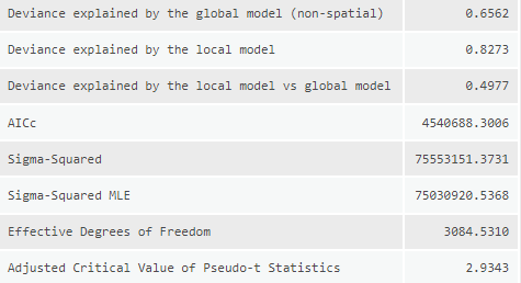
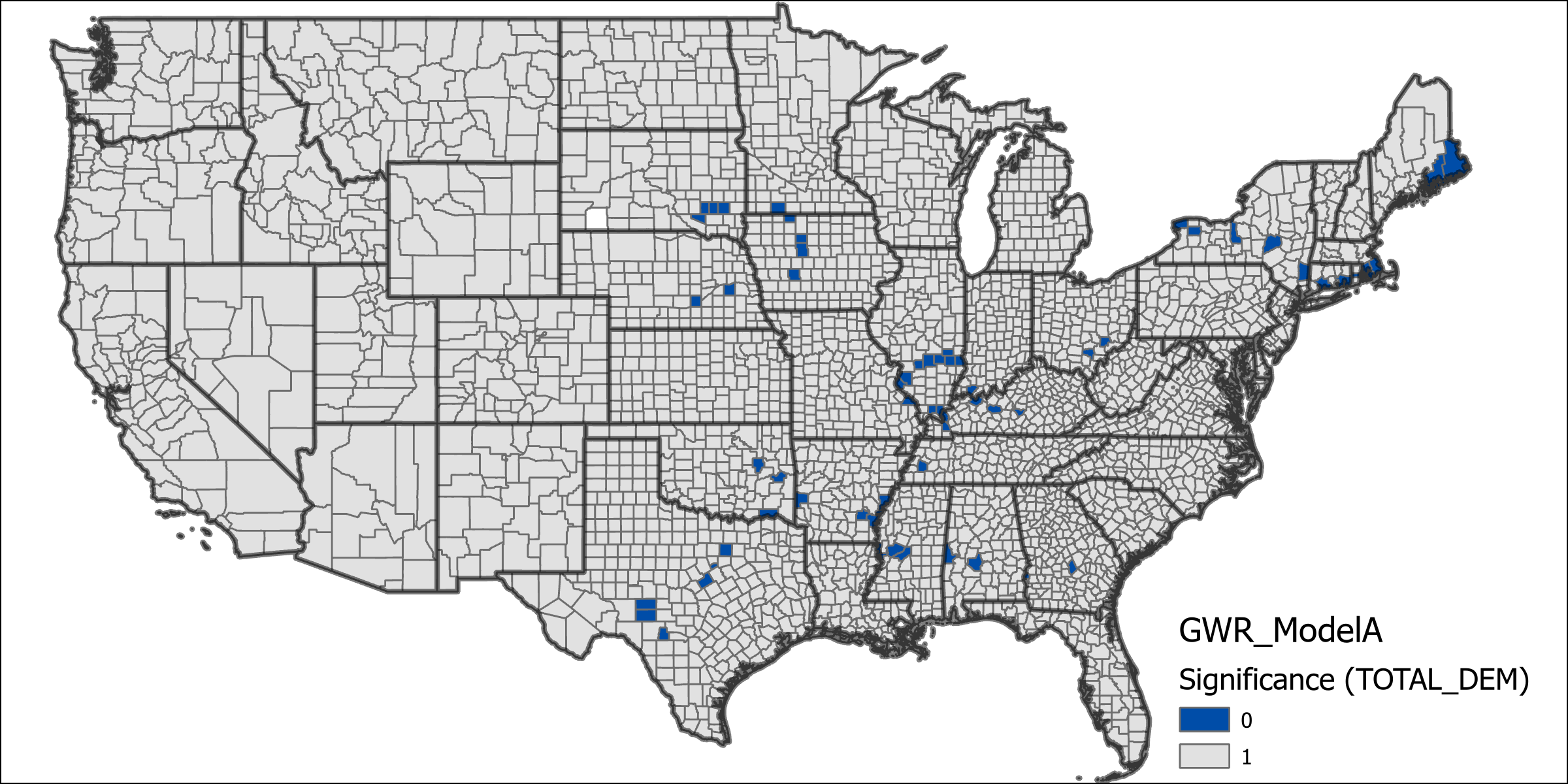
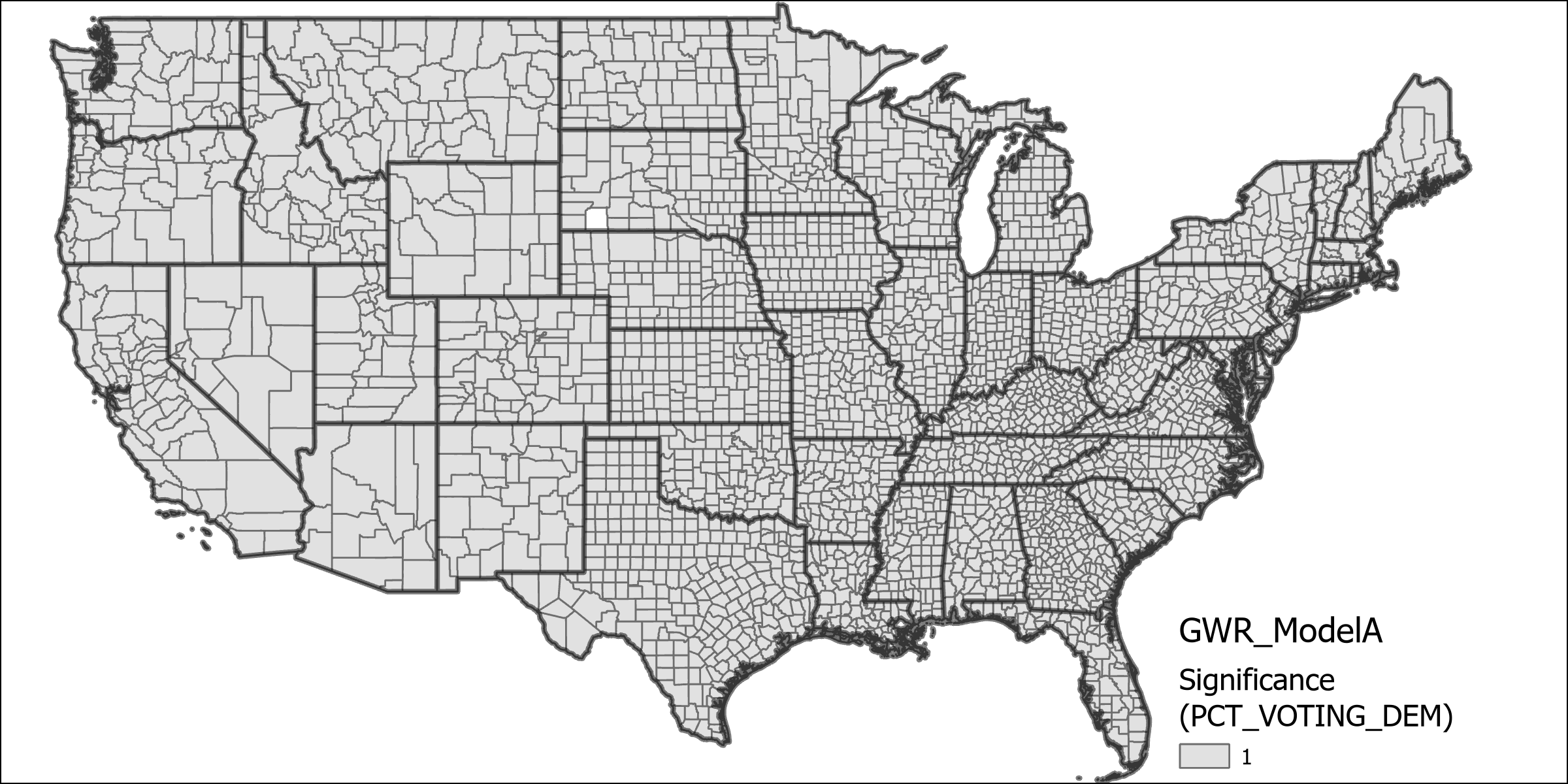
The table below shows the results from running model A. There is a very high degree of deviance explained by the local model (0.8273), showing significant improvement over it’s global model. Further we can see from the two below maps that both state-level democratic immigration rates and county level democratic voting percentages have statistical significance in nearly every county. From the coefficients of the model we can see that the state level immigration count contributes the most to the model, followed by median age, population density then county voting percentages.

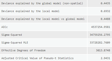
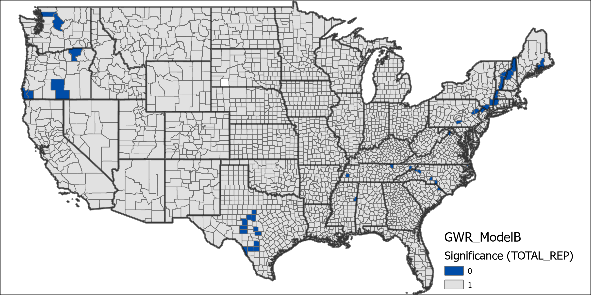
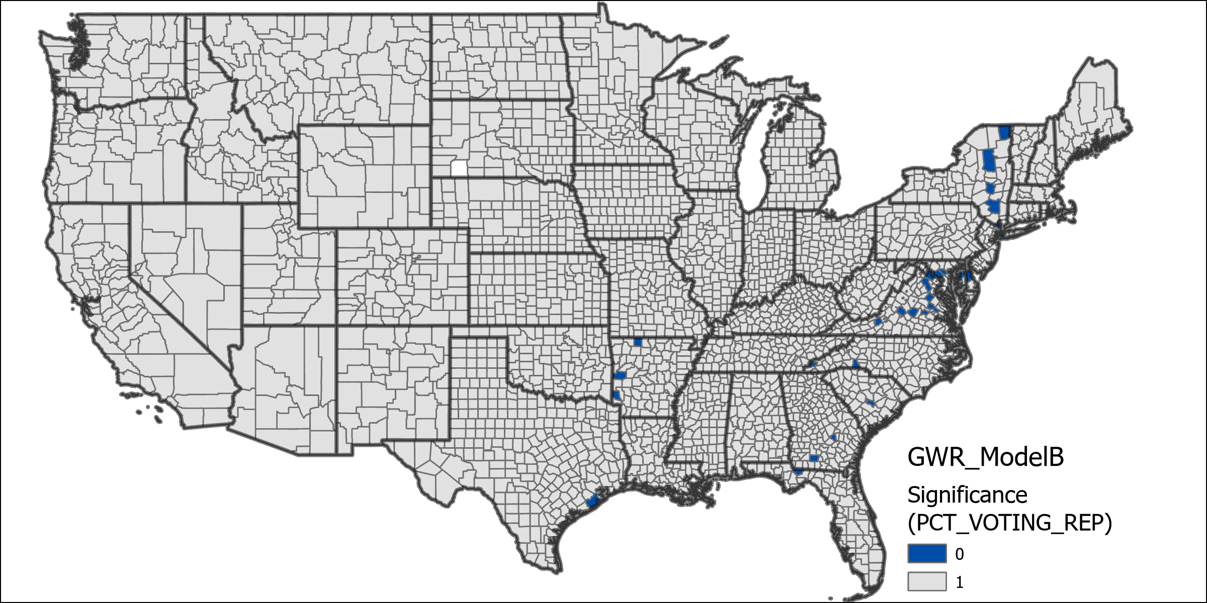
Model B did not perform nearly as well as model A, with a total deviance explained of 0.6932, which is still a relatively high amount of deviance explained by the model. The difference between these two models supports the notion that local origin characteristics can have a predictable impact at the destination. It would appear that migration from republican voting counties is not as predicable (using these estimation variables) as democratic counties. Looking at the maps of variable significance we can it present in most counties, but not as many as in model A. From the chart of coefficients we can see that county voting percentage is now the most significant contributor to the model while state level migration count does not contribute as much.

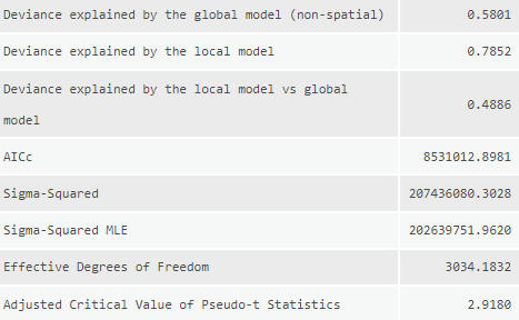
In model C only democrat voting percent is utilized because it is too closely related to the republican voting percentage (although there are votes for other candidates, they don’t make up a significant number), as such it can be reasonably assumed the addition would not affect this model much (it assumes that the republican voting percent is the inverse of democrat). Unsurprisingly the deviance explained by this model lies between Models A and B at 0.7852. Maps of significance for the variables tested by this model indicate high overall significance for all variables. The chart of coefficients has a diminished effect on state level migration counts compared to model A, while also exhibiting the enhanced effect of county level voting percentages from model B.

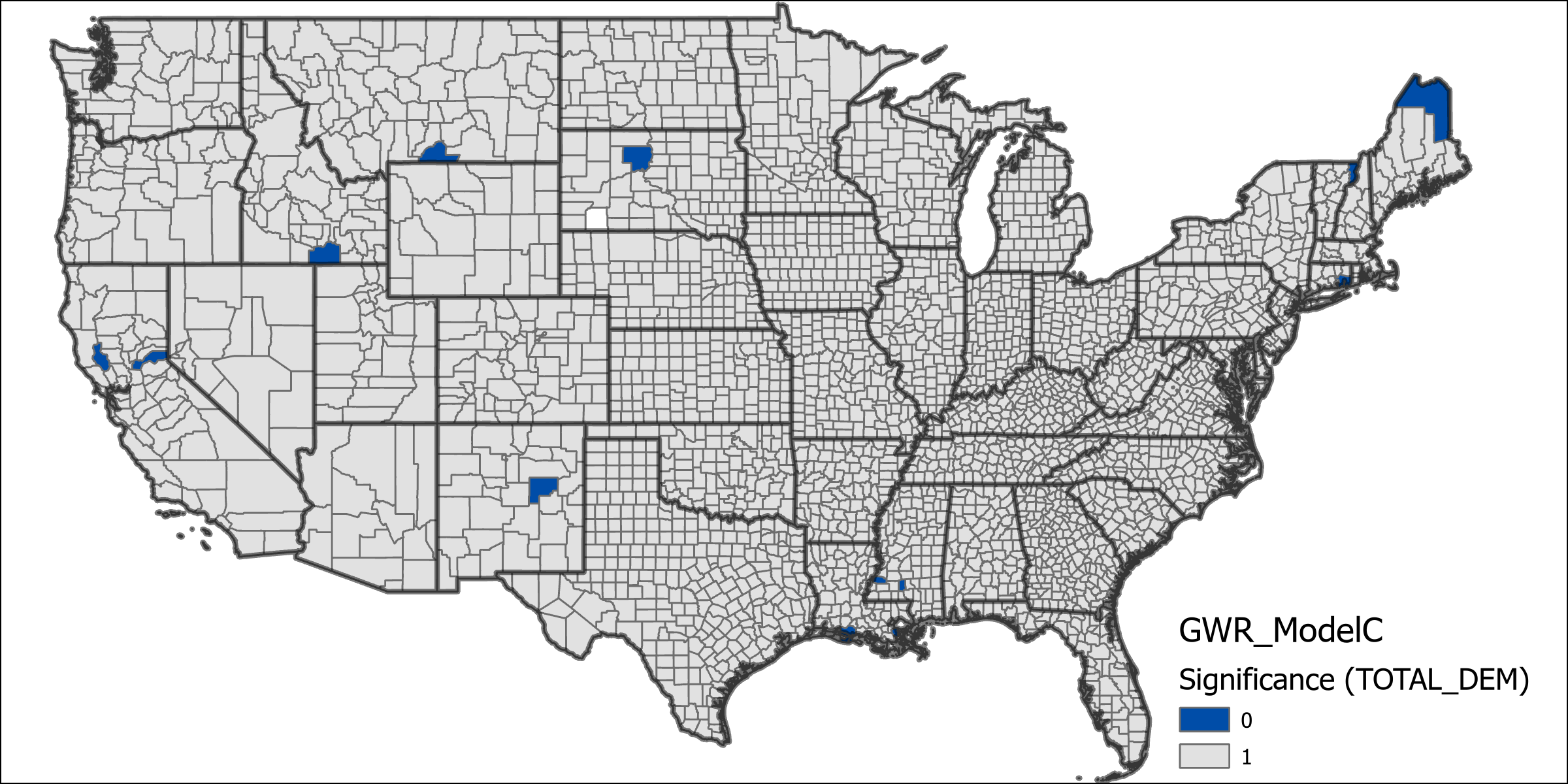
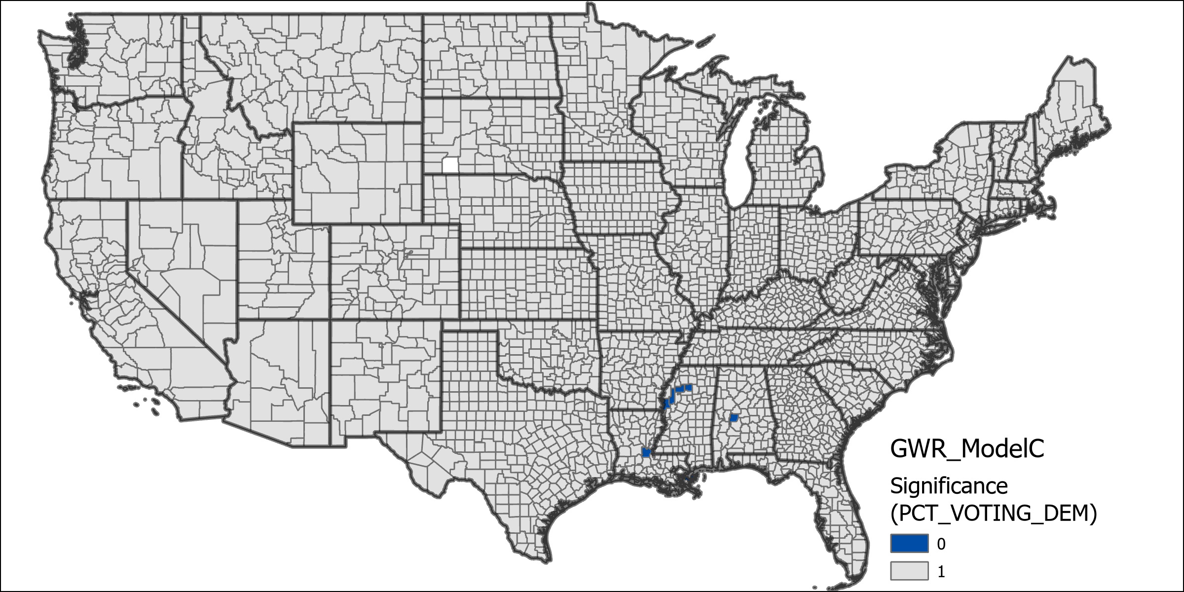
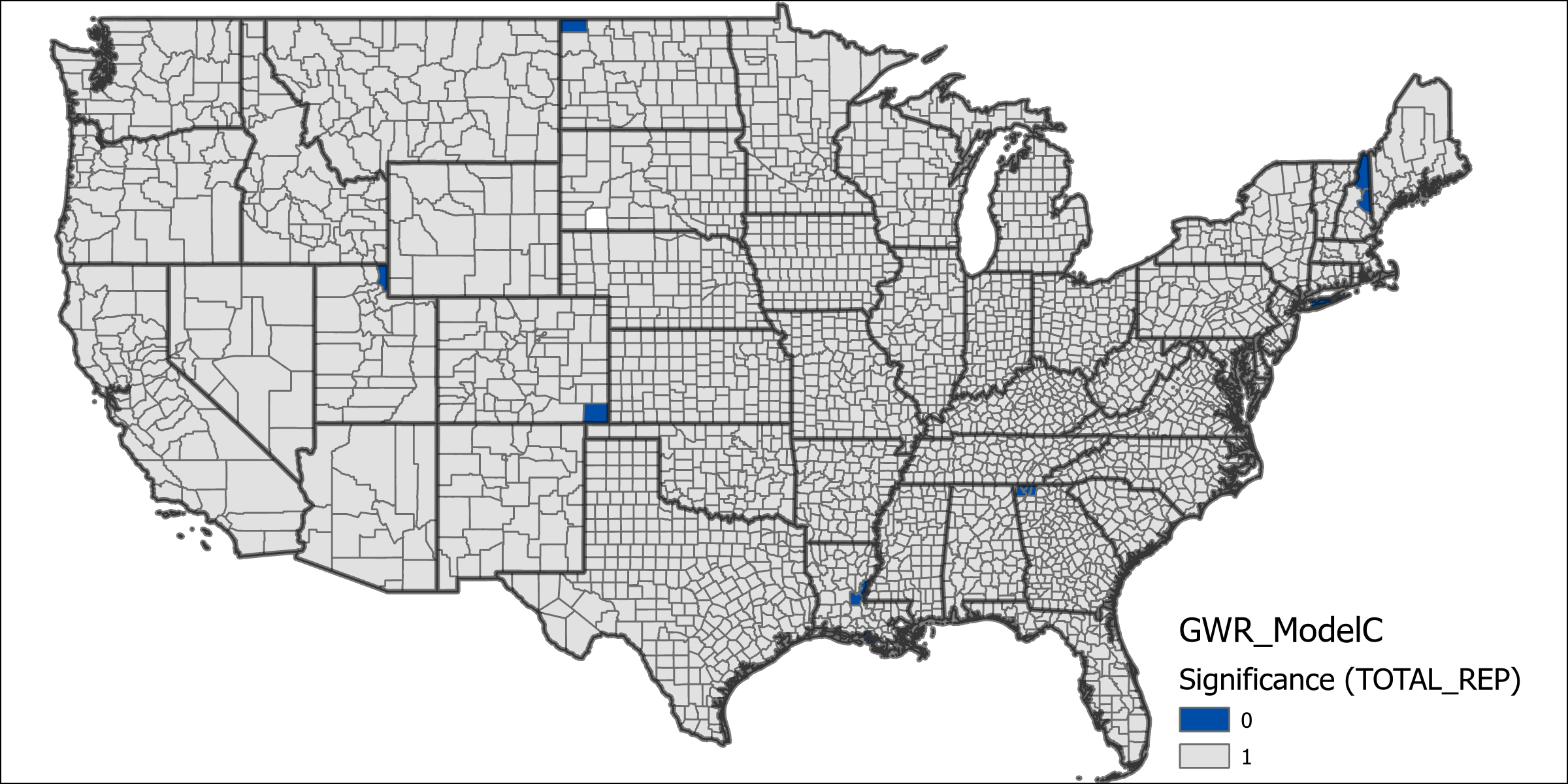
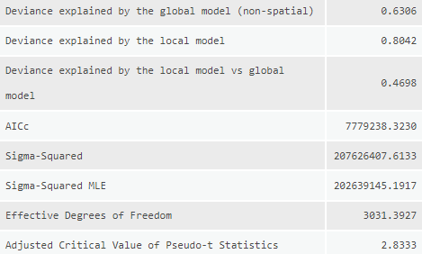
The “Far” and “Very Far” distance grouping variables are precluded from Model C because there are a number of states which have no corresponding states in these groupings that are clustered together which would prevent the model from running. This model shows an increase in the explained deviance over model C, however still less than model A at 0.8042. This model can be further compared to model C using the AIC values which is significantly lower. The increase in explained deviance between models indicates that the distance for migration at least accounts for some of the deviance. The table of significance counts for the values shows that the variables individually have less significance across more counties in this model. The increased number of variables makes it more difficult to compare the differences in coefficients for this model, although it does exhibit similarly high values for county level voting rates as in models B and C.
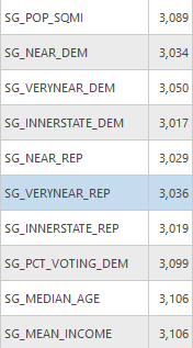
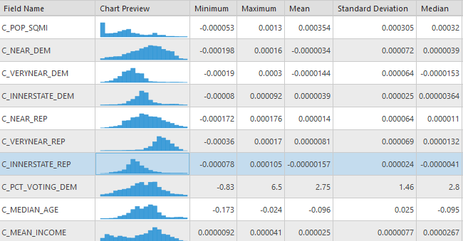
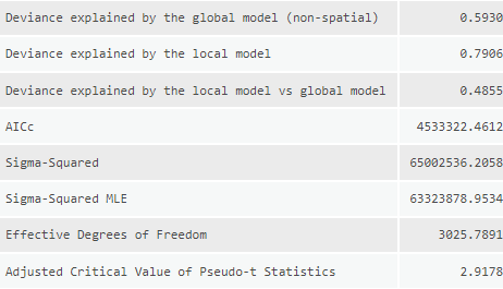
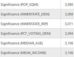
When compared to model D, model E shows a slight degradation in explained deviance at only 0.7906. The model shows slightly improved significance rates for state level migration trends, but still poorer than models A-C. There was no significant difference in coefficient values compared from model D and E.
Based on the results from the above models I create a final model “P” that combines aspects from model A and model D in order to create the most predictive model possible. Using this model I also created prediction values to determine the overall accuracy of the model. The prediction input features are the same county features used to create the model. This model excludes states that do not have “Far” states so that the “Far” grouped migration counts can be added to the model.
| Model P | DV: Estimated Democrat Immigration, IVs: Democrat voting rate, Democrat Immigration at various distances (4 variables – Innerstate, Very Near, Near and Far), population density, age and income |
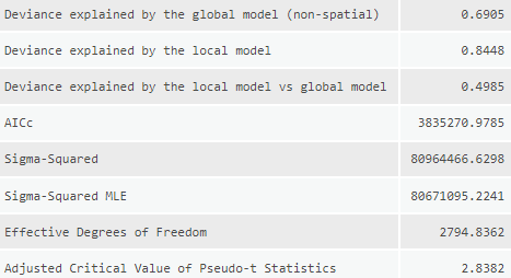
The results from Model P shows a greatly improved explained deviance compared to the other models. Additionally it has a significantly lower AIC value compared to Model A.
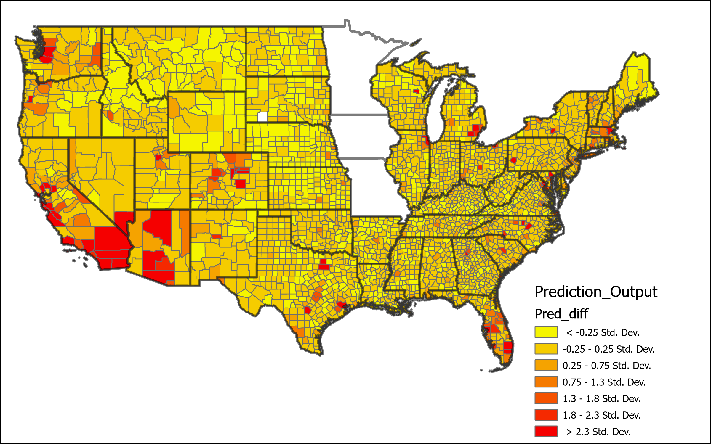
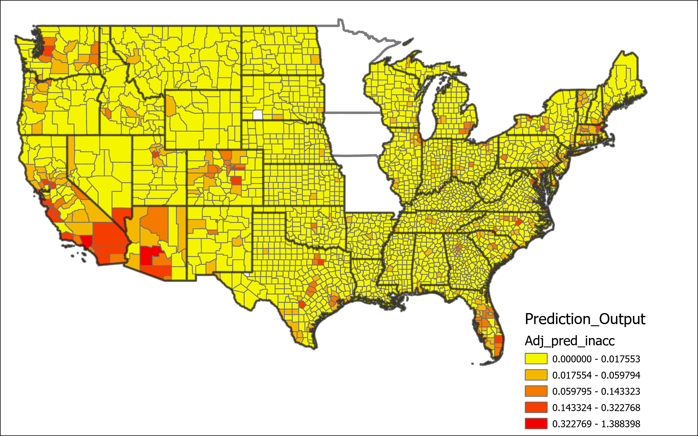
In order to determine the scale of inaccuracy in the model prediction I calculated a few variables to check the closeness. First I calculated the difference between actual and expected values. This value shows how far off the numbers are, however counties with higher migration numbers are bound to have a larger difference, even if the model is more accurate for that county. Next in order to find the scale of difference relative to the size immigration I used the simple formula of inaccuracy rate = ( | predicted value – actual value |) / actual value to determine how far off the prediction is relative to the size of the value. As might be expected this variable shows a high rate of inaccuracy for smaller counties where small differences of less than 50 can create incredibly high rates in the 1000%s or more. Finally I create an adjusted inaccuracy rate which is calculated using adj. Inaccuracy rate = inaccuracy rate * (actual value/143283) where 143283 is the maximum actual value for any county. Based on this adjusted variable counties will have an inaccuracy representative of their relative size compared to other counties, small counties will not be weighted as heavily, while the largest county will maintain the same inaccuracy rate.

Results
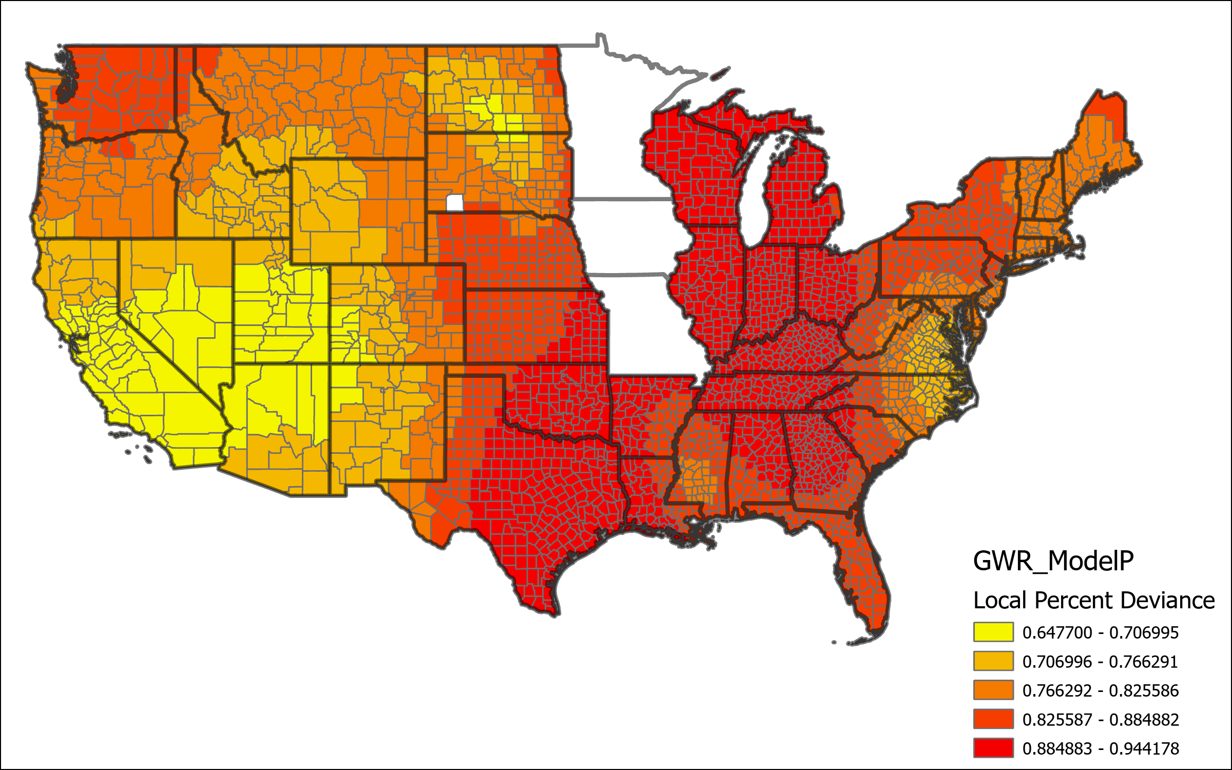
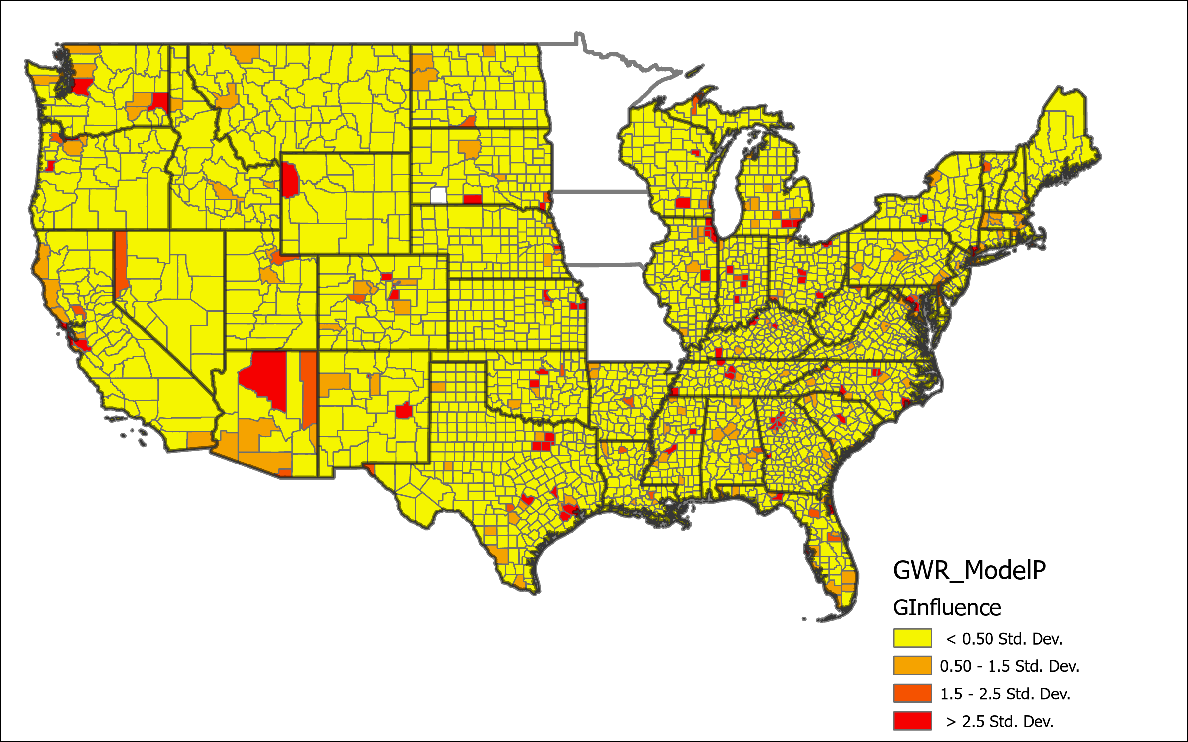
The map above represents the Local percent deviance from Model P. This shows the counties which are best predicted, or not predicted, using this model. There is clear lower levels of local percent deviance located predominantly in Southwest states, and also in the Dakotas and the coastal border of Virginia and North Carolina. Other geographic areas represent a much higher degree of certainty, a significant portion even around 90% local deviance explained by the model. Based on this result we can determine determine that this model is likely missing some key variables that would give better explanation for the deviation in the low percentage areas. Further the map of Geographic Influence below shows what appears to be a random distribution of high and low values across the country, indicating that local estimations are well fit according to spatial variations within the global model.
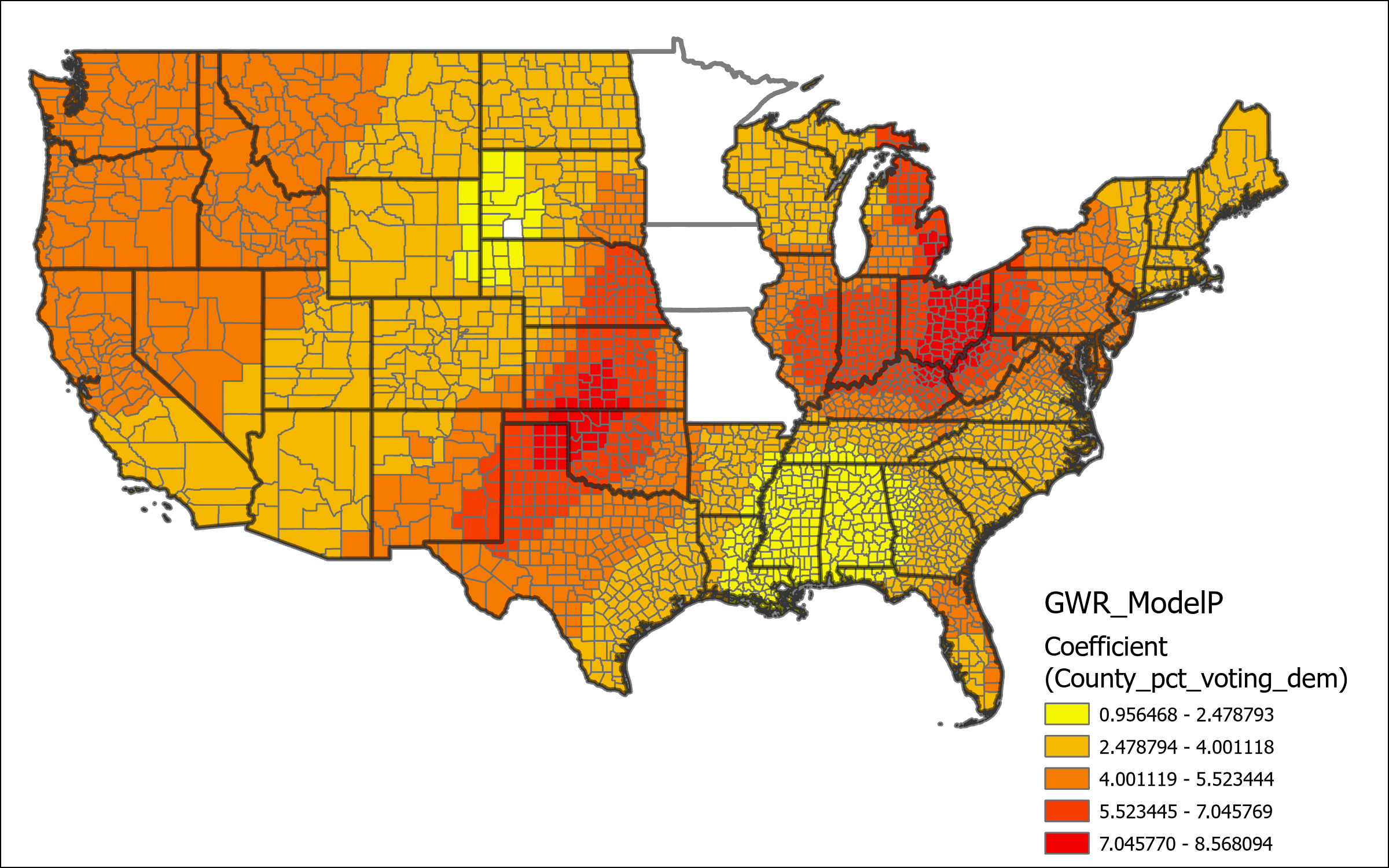
We can further look at maps of some of the key coefficient values to determine the impact that those variables have on the model at the local level. The coefficient for the variable indicating the counties percent of population for Biden in the 2020 general election shows some key details. First based on the the fact that the coefficient is positive in all cases we can determine that emigrants from democratic voting counties have a greater propensity to immigrate into democratic voting counties. The effect of this propensity is most pronounced in the Central and Midwest Regions, with the least explanation in the Gulf Coast and in South Dakota.
Next we can take a look at the coefficients for state level migration trends. This model separates the state level migration based on categorical distance from the origin state, as such we can compare the maps of each of these coefficients directly to determine the impact that distance may have in different areas.
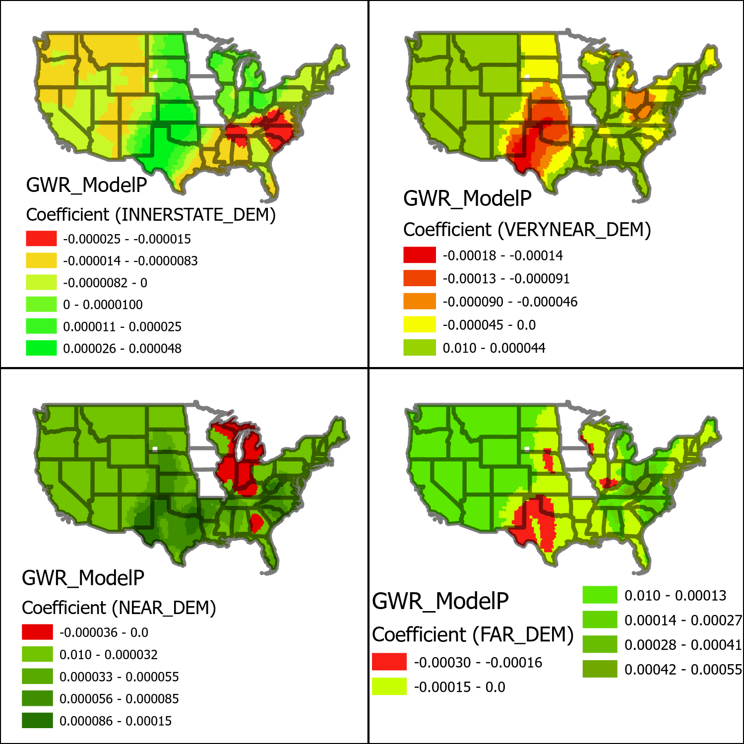
From these maps some interesting patterns start to emerge. For starters each variable seems to have a geographically distinct profile separate from the other variables. These variables also have the interesting characteristic that they flip from negative (red-yellow) to positive (green) values depending on the geographic context. The negative coefficient areas indicate that greater levels of migrants coming from democratic voting counties results in fewer of those immigrants moving to the county, presumably this is explained by greater positive relationships to the other distance variables. The innerstate map a distribution of efficacy that seems to be very closely related coefficient model for county voting percentages. The very near map on the other hand seems to be a nearly exact opposite from the interstate map, indicating that very near migration accounts for the majority of deviance that innerstate migration does not. The near and far migration maps seem to be more generally positive indicating that there is generally very little interference in explained deviance from the other two closer distance groups on these two farther categories.

Lastly we can look at the coefficient value maps for the more generic explanatory variables from the maps above. Uniformly across the country population density and mean income are positively correlated while median age is negatively correlated. This suggests that immigrants from democratic voting counties are more likely to move to counties with greater population density, higher income, and with younger populations. Population density has a greater effect on the model around the Gulf Coast, Income around the center of the U.S. and age around the Midwest. The distribution on the efficacy of these variables seems to geographically independent of the other explanatory variables.
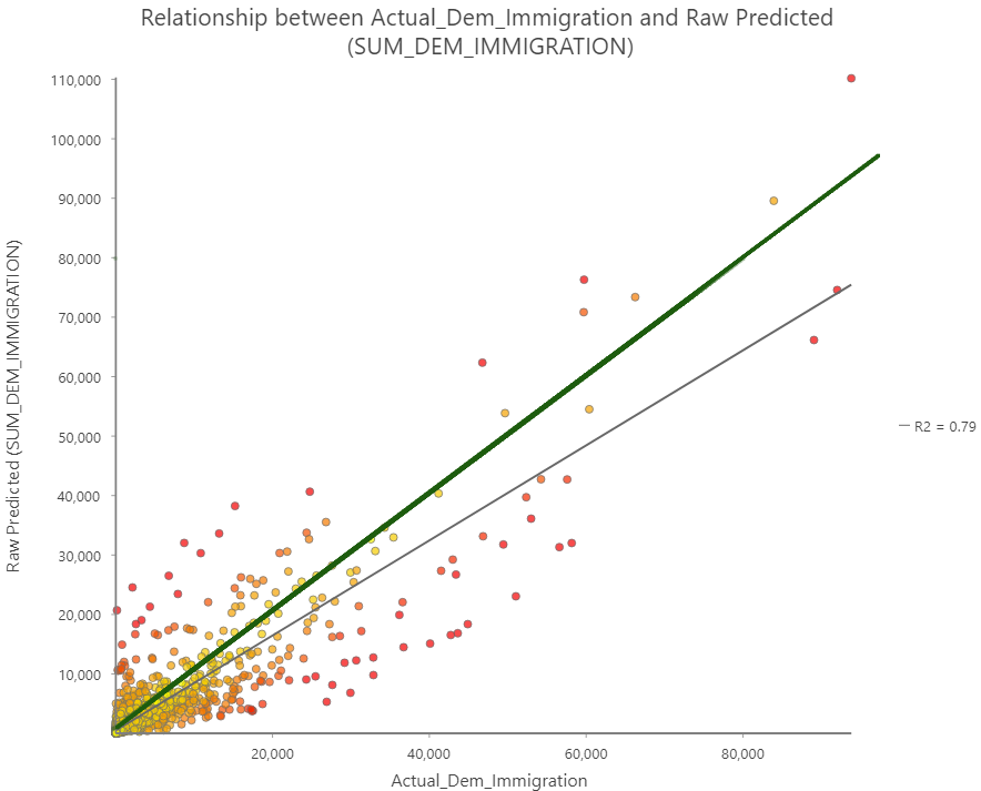
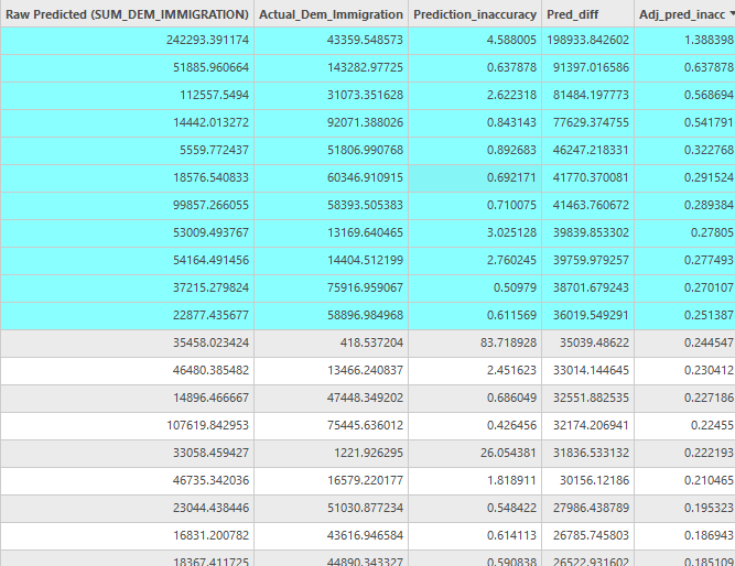
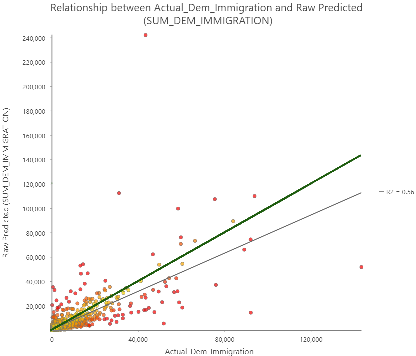
In the scatterplot above the relationship between the actual migration values and the predicted values computed by the model can be examined. The green line represents a one to once relationship between predicted and actual values, the values closest to this line are the most accurate. The gray line represents the actual trend line of the scatterplot data. The R2 value is only 0.56 indicating a that model tends to heavily under predict the values. Looking at the individual counties from the prediction analysis it can be determined that there is generally decent levels of accuracy when using the adjusted inaccuracy, with the exception of only a small number of outliers that have values above 0.2, highlighted in the table below. These outliers are very spatially clustered and are representative of the same areas where the regression model has the lowest values for explained deviance. This is unsurprising as these areas should be to have the highest degree of inaccuracy. Filtering these outliers from the data produces a much tighter scatter plot and a more accurate trend line, although there is still a tendency in the model to underpredict values.
The complete output from GWR Model P and Prediction results are available below in the interactive map.
Considerations and Discussion
There are several big caveats to this research that needs to be addressed up front. There is significant potential error due to not having access to individual level data, in particular the use of aggregate voting characteristics instead of individual ones. It is important to recognize that the impacts of individual characteristics cannot be inferred from this model, only the impact of small aggregate characteristics from an individuals origin.
From this data there is a clear connection between the county level political characteristics and migration destination selection. An important thing to consider however is that more democratic counties tend to have larger populations. This can in fact be pointing towards what we already know from the gravity model, people from large settlements will tend towards moving towards other large settlements, an attribute that is especially pronounced over distance. Since the accuracy of the model decreased when looking at more local migrations this seems to be a likely possibility. Additionally we can consider the failure of model B, using Republican migration estimates instead of Democratic resulted in a less predictive model primarily due to a decrease in the applicability of national migration trend estimates, however the effects of destination unit characteristics became more pronounced. This finding could support Tam Cho et Al (2012)’s finding that Republicans and Democrats are similarly likely to migrate to large cities while Republicans are more likely to migrate out of those cities to nearby suburbs or rural areas, while Democrats are more apt to stay. This migration pattern calls into question the utilization of only local level data to determine political polarization, it may be the case that new immigrants are constantly mixing when moving long distances, and then progressively sorting themselves after becoming more acclimated. A local level only analysis misses the potential impact of outside sources. The data supports this possibility since the migration patterns have different effects depending on the distance that was traveled. Further longitudinal analysis with individual characteristics across large dimensions of space will be required in order to analyze this possibility or determine if there is other factors influencing the independent variables used here.
One other major drawback comes from the prediction methodology that was utilized. In order to create a predictive model it was necessary to know or estimate the end result. This limits the potential use of predictive analysis to only model persistent trends. If new trends are initiated, such as through unique migratory impacts like economic downturns, political chaos or health crises, it would be possible to detect the new trend using GWR, however it will be necessary to wait until some actual results have been established before a prediction model can be employed. This waiting period would make tracing the impact of single time events, like a storm, impossible to predict.
One important consideration with this model is that the 2016-2020 period has been noted by some observers to be an especially turbulent political time in the U.S. If this is indeed a unique period in the U.S.’s future then the significance of political characteristics in migration data may soon come to an end. It would be interesting to see how this form of model might be adapted to other variables tracking migration during other turbulent events, such as economic downturns or health crises. It may be possible that the impact of certain variables can be predicted by their migratory impact in other historic events, for instance one could input financial variables from a recession in the 20th century and see if there are maintained for similar recessions in the 21st century. This may be one way of overcoming the temporal nature of predictive models.
One thing is made clear by this study, it is possible to use characteristics from small data units in order to create accurate predictive models using only larger aggregate units. Although the accuracy of this particular model is questionable due to the estimated nature of the small unit characteristic data, such methodology may be useful in creating multi-level analysis in the future. One example may be new state level abortion laws that may trigger a particular political party to migrate in higher levels than other political parties. A survey can be conducted asking respondents simply if then intended to migrate and their current political affiliation, this data could then be aggregated to larger units without revealing any private details and still utilize a formerly created predictive model to determine where immigration will be likely to occur and provide necessary resources to those locations.
References
Literature
Tarver, J. D. (1961). Predicting Migration. Social Forces, 39(3), 207–213. https://doi.org/10.2307/2573210 Poot, J., Alimi, O., Cameron, M.P. and Maré, D.C. (2016) The Gravity Model of Migration: The Successful Comeback of an Ageing Superstar in Regional Science. IZA Discussion Paper No. 10329. http://dx.doi.org/10.2139/ssrn.2864830 Lam, K, (2002). Interaction between Economic and Political Factors in the Migration Decision. Journal of Comparative Economics,30(3), 488-504. https://doi.org/10.1006/jcec.2002.1783 McHugh K.E. and Gober, P. (1992), Short-Term Dynamics of the U.S. Interstate Migration System, 1980–1988. Growth and Change, 23: 428-445. https://doi.org/10.1111/j.1468-2257.1992.tb00943.x Rogers, A. and Raymer, J. (2001) Immigration and the Regional Demographics of the Elderly Population in the United States. The Journals of Gerontology: Series B, S44–S55, https://doi.org/10.1093/geronb/56.1.S44 Dennett, A., & Wilson, A. (2013). A Multilevel Spatial Interaction Modelling Framework for Estimating Interregional Migration in Europe. Environment and Planning A, 45, 1491 – 1507. Liu X, Andris C, Desmarais BA (2019) Migration and political polarization in the U.S.: An analysis of the county-level migration network. PLOS ONE 14(11): e0225405. https://doi.org/10.1371/journal.pone.0225405 Tam Cho, W.K., Gimpel, J.G., & Hui, I.S. (2012). Voter Migration and the Geographic Sorting of the American Electorate. Annals of the Association of American Geographers, 103, 856 – 870. Badger, E., Quealy, K., & Katz, J. (2021, March 17). A Close-Up Picture of Partisan Segregation, Among 180 Million Voters. The New York Times. https://www.nytimes.com/interactive/2021/03/17/upshot/partisan-segregation-maps.htmlData
U.S. Census Bureau. (2020). County-to-County Migration Flows: 2015-2019 ACS. [Data file]. Retrieved from https://www.census.gov/data/tables/2019/demo/geographic-mobility/county-to-county-migration-2015-2019.html MIT Election Data and Science Lab, 2018, "County Presidential Election Returns 2000-2020", https://doi.org/10.7910/DVN/VOQCHQ, Harvard Dataverse, V10, UNF:6:pVAMya52q7VM1Pl7EZMW0Q== [fileUNF] U.S. Census Bureau, ESRI (2020). 2020 USA Census Counties. [Data file]. Retrieved from https://services.arcgis.com/P3ePLMYs2RVChkJx/arcgis/rest/services/USA_Census_Counties/FeatureServer U.S. Census Bureau, ESRI. (2020). 2020 USA Census States [Data file]. Retrieved from https://services.arcgis.com/P3ePLMYs2RVChkJx/arcgis/rest/services/USA_Census_States/FeatureServer U.S. Census Bureau. (2020). 2020 American Community Age and Sex 5-Year Estimates [Data file]. Retrieved from https://data.census.gov/cedsci/table?q=mean%20age%20by%20county%20in%202020&tid=ACSST5Y2020.S0101 U.S. Census Bureau. (2020). 2020 American Community Mean Income In The Past 12 Months (In 2020 Inflation-Adjusted Dollars [Data file]. Retrieved from https://data.census.gov/cedsci/map?q=mean%20income%20by%20county%20in%202020&tid=ACSST5Y2020.S1902&cid=S1902_C03_001E&layer=VT_2020_050_00_PY_D1&mode=thematic&loc=19.4169,-101.3671,z3.0000Tools
ESRI (2022) ArcGIS Pro (Version 3.0) [Computer software]. https://www.esri.com/en-us/arcgis/products/arcgis-pro/overview ESRI (2022) Geographically Weighted Regression (GWR) [Python script]. https://pro.arcgis.com/en/pro-app/latest/tool-reference/spatial-statistics/geographicallyweightedregression.htm#L_Reflection
Overall I was not able conduct this research to the full extent that I had hoped, however I was still able to turn up interesting results. The lack of small unit data that could be easily connected to characteristics was a particular pain point for me trying to solve. One thing that didn’t work out the way that I had anticipated was the incorporation of distance measures, although I wanted to use fixed distances for the data, I hadn’t considered that it would make states unusable if they didn’t have sufficient neighbors at that distance level to draw upon. One way that I might now fix the distance grouping variable is to group based upon the nearest neighbors instead of a fixed unit. This would prevent any unit from not having any neighbors for the distance group. I was particularly interested by the possibility of differing scale migration flows accounting for Republican polarization, as it wasn’t really a result that I was anticipating before actually looking at the data that was returned. I learned a great deal about setting up variables for GWR analysis as well, I hadn’t intended to create more than one GWR model but I quickly discovered that I wasn’t going to be able to create an optimal model without first performing some different tests.
